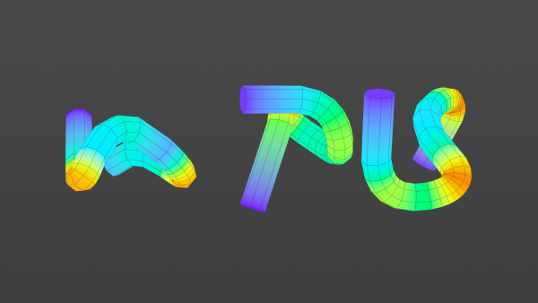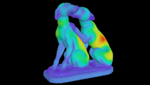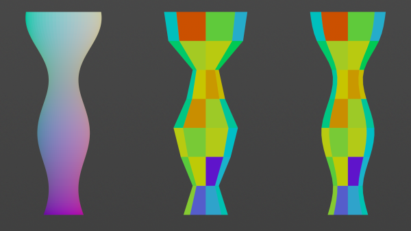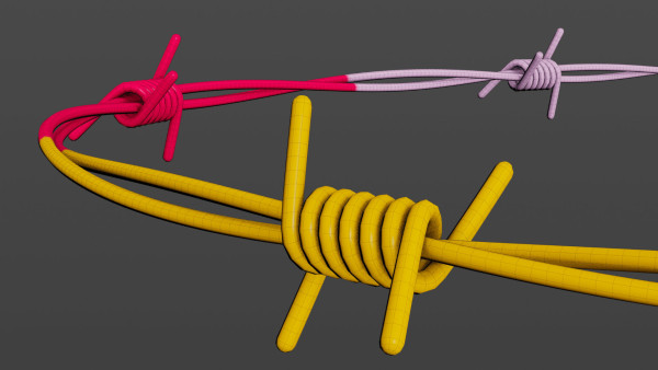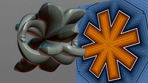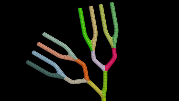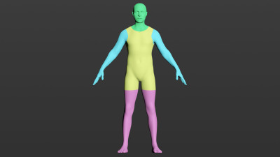
Segmenting meshes based on eigen vectors created by the laplacian node and the linear solver.
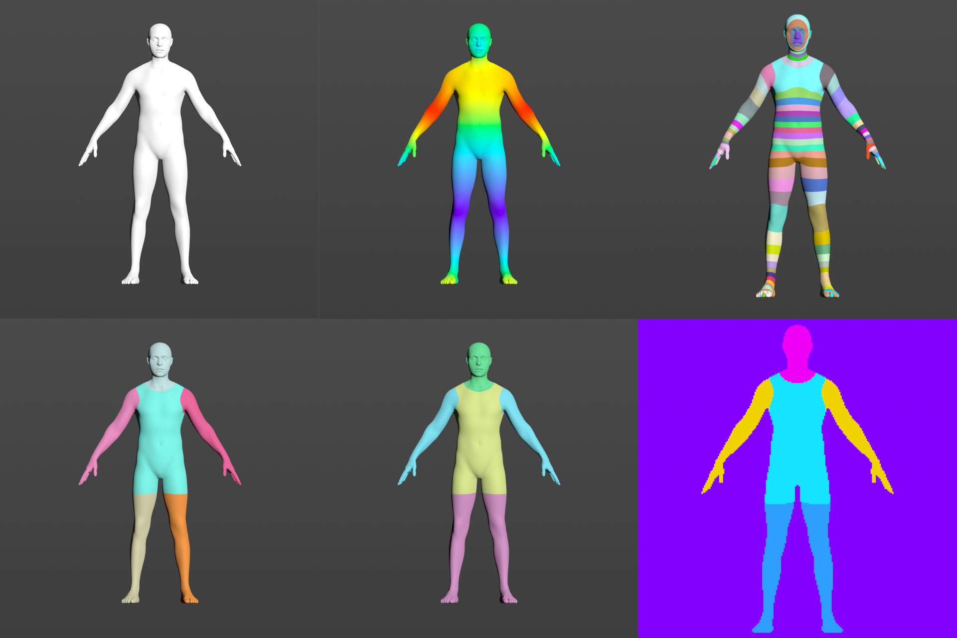
The input mesh (1) is split into bands (3) based on a cyclically remapped eigenvector (2) found by the linear solver. Neighbouring pieces are then combined to segments (4) if their measured quantities such as perimeter or area are similar defined by a threshold inside the group from attribute boundary-node. Segments with similar quantities are additionally put into their own class (5) using the fuse-node.
The segmentation procedure has many options for adjusting bands, segments and combining classes. The result is a segmented mesh along with a segmented image (6) suitable for machine learning.
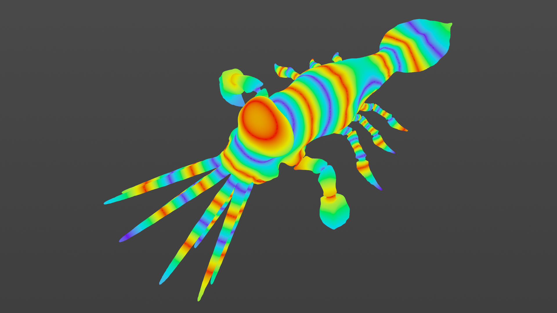
In abstract terms, the Laplacian Node describes neighborhood relationships between mesh points. “col” contains the neighboring points as well as the point's own number, while ‘mass’ and “value” weight their respective significance within the network. The Linear Solver calculates eigenvectors based on this. Its SymEigsShiftSolver induces mutually offset oscillations throughout the entire mesh to measure where these oscillations are dampened by curvatures or other high-frequency regions, as defined by “mass” and “value.” This results in very smooth eigenvector maps, which can be cyclically remapped to slice the mesh into bands.
These bands are then recombined into segments based on similar metrics for area, perimeter, or curvature. Furthermore, the fuse node can group the centroids of segments with similar quantities into common classes regardless of their world position, so that the torso, head, arms, and legs each end up in their own classes. The final step would then be the automatic naming of the classes using AI, which receives a ray-traced image of the segmented and class-assigned mesh in order to place names on it.